This article explains the behavior of LASTNONBLANK, LASTNONBLANKVALUE, and similar DAX functions, also providing patterns for performance optimization.
The DAX language can operate on aggregated values and on individual rows of tables in the data model, but it does not offer an immediate syntax to perform visual-level calculations over the cells visible in a report. The reason is that a DAX measure must work in any condition and in any report, which is why the notion of row context and filter context exists in the DAX language.
When you need to apply the notion of “first”, “previous”, “next”, “last” while iterating a table, you might have to struggle with these concepts in order to get the result you want. There are a few DAX functions that can simplify the syntax, but they must be used with caution in order to not hurt the query’s performance:
- FIRSTNONBLANK
- FIRSTNONBLANKVALUE
- LASTNONBLANK
- LASTNONBLANKVALUE
This article explains how these functions work, how to use them correctly, and how to apply optimizations resulting in DAX code that does not use these functions at all!
Comparing with previous value
The Contoso model we use contains sales transactions where a customer has different orders on different dates. Each order can include multiple transactions and there can be multiple orders from the same customers on any one date. We analyze two scenarios:
- Sales PD: Compare the Sales Amount of one day with the previous day
- Sales PO: Compare the Sales Amount of one order with the previous order.
Because these calculations are dynamic, by filtering one customer the comparison only occurs considering the days and orders where there are transactions for that filtered customer. The dynamic nature of this calculation makes it very expensive to pre-calculate such amounts.
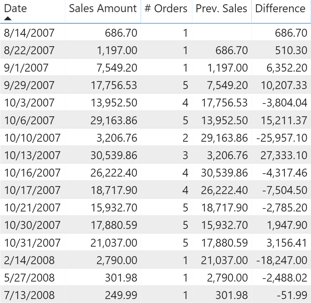
The first example compares one day with the previous day available by filtering the transactions of one customer.

The challenge is to find the previous day, and then retrieve the value of that day. Because one day can have multiple orders for one same customer, the calculation must operate at the day granularity level.
The second example is a similar report where we have one row for each order instead of one row for each day. The following visualization only shows the first orders made by the customer.
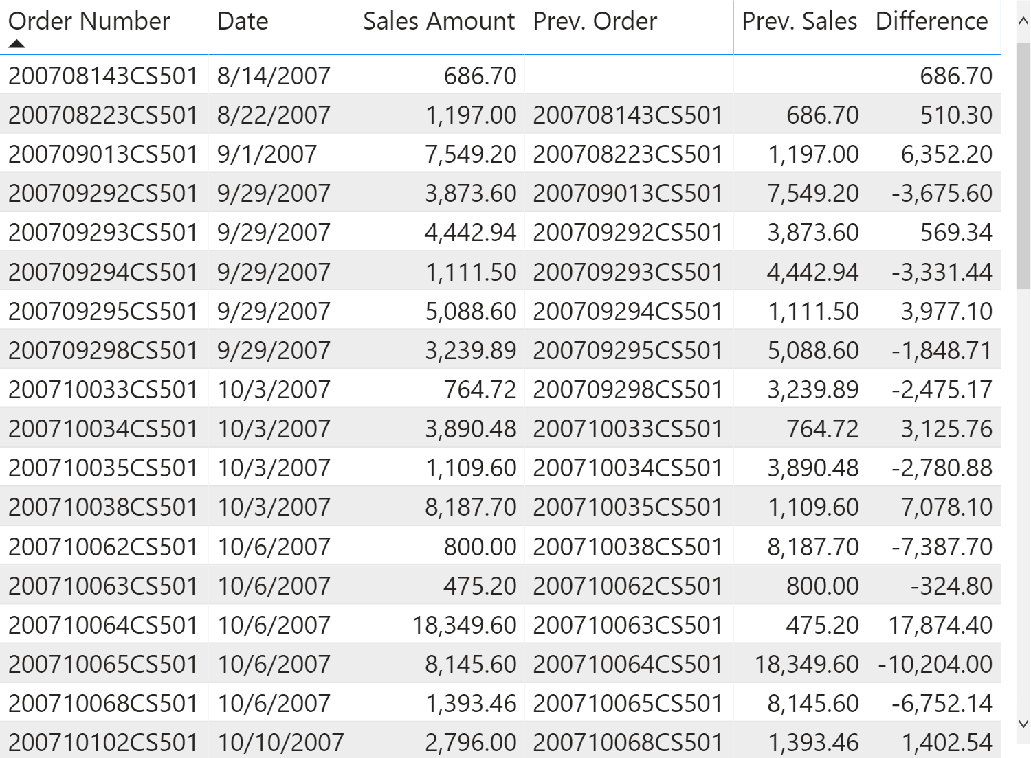
In this case, the calculation must be done working at the order granularity level, which is still an aggregation of one or more transactions.
Understanding FIRSTNONBLANK and LASTNONBLANK
The Sales PD scenario requires implementing the following business logic in a measure:
- Retrieve the previous date when there are transactions in the current filter context.
- Evaluate Sales Amount filtering the date found in the previous step.
We can implement the first step using the LASTNONBLANK function as shown in the Prev. Order Date v1 measure:
Prev. Order Date v1 :=
IF (
    NOT ISEMPTY ( Sales ),
    VAR FirstVisibleDate =
        MIN ( 'Date'[Date] )
    VAR PreviousDate =
        CALCULATE (
            LASTNONBLANK (
                'Date'[Date],
                [Sales Amount]
            ),
            'Date'[Date] < FirstVisibleDate
        )
    VAR Result =
        IF (
            NOT ISEMPTY ( Sales ),
            PreviousDate
        )
    RETURN
        Result
)
The LASTNONBLANK function iterates all the values in the column provided as the first argument. For each value it evaluates the expression provided in the second argument, returning the largest value included in the first argument that generated a non-blank result as it was evaluating the expression provided in the second argument. In this case, the Sales Amount measure is evaluated for each date in the filter context. Because we need to retrieve the last date with a transaction made by one same customer filtered in the report, we have to modify the filter context for the Date table; otherwise, for each cell of the report we would only consider the date of the current line in the report. This is the reason why the LASTNONBLANK function is wrapped inside a CALCULATE function that filters only the date before the date visible in the cell of the report:
CALCULATE (
    LASTNONBLANK (
        'Date'[Date],
        [Sales Amount]
    ),
    'Date'[Date] < FirstVisibleDate
)
When LASTNONBLANK is executed providing a column reference as the first argument, DAX implicitly rewrites the expression by retrieving the values using DISTINCT in a potential context transition. The previous code is internally rewritten as:
CALCULATE (
    LASTNONBLANK (
        CALCULATETABLE (
            DISTINCT ( 'Date'[Date] )
        ),
        [Sales Amount]
    ),
    'Date'[Date] < FirstVisibleDate
)
You can also provide a table as a first argument of LASTNONBLANK. Thus, the same expression could have been written as:
LASTNONBLANK (
    CALCULATETABLE (
        DISTINCT ( 'Date'[Date] ),
        'Date'[Date] < FirstVisibleDate
    ),
    [Sales Amount]
)
The FIRSTNONBLANK function is identical to LASTNONBLANK, with the only difference that it returns the smallest value instead of the largest value included in the first argument that generated a non-blank result when evaluating the expression provided in the second argument.
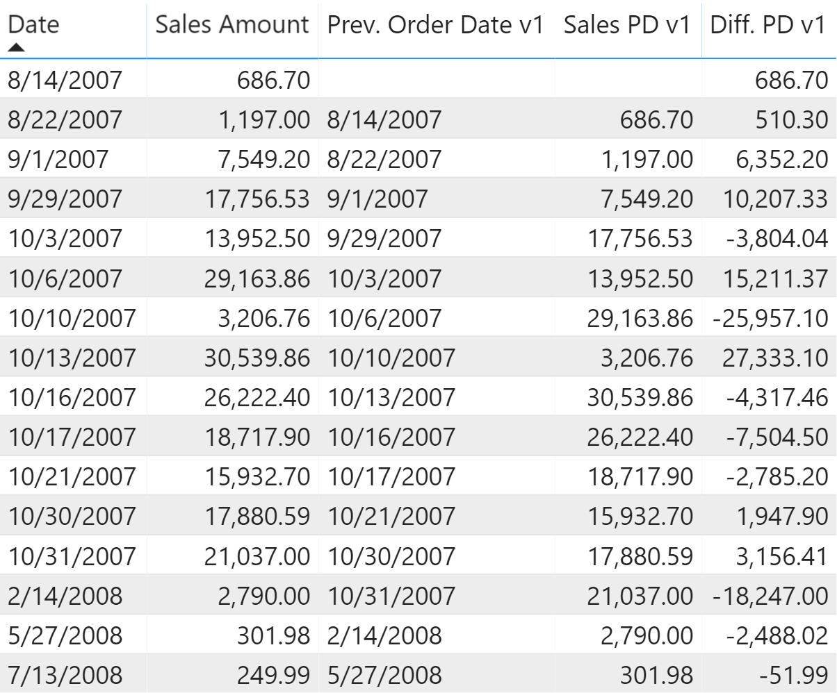
The following screenshot shows the result of the Prev. Order Date v1 measure. As expected, this is simply the date of the previous line in the report.
However, if you give some thought to the work that must be done, LASTNONBLANK and FIRSTNONBLANK could potentially iterate a large number of rows. When we filter all the dates before a certain date, the number of rows considered could be in the order of thousands if you have a Date table with 10 years, and this must be repeated for every cell in the report. In order to avoid this useless task, the Prev. Order Date v1 measure offers an important optimization: it executes the search if and only if the current filter context has rows in the Sales table:
IF (
    NOT ISEMPTY ( Sales ),
    ...
This means that in the previous report the LASTNONBLANK function is only executed 16 times instead of hundreds of times because of the several years available in the model. This way, we also avoid displaying a previous order date for dates when there are no transactions.
Now we can implement the second step of the calculation. The date obtained by the Prev. Order Date v1 measure can be used as a filter to retrieve the Sales Amount value on that date. The Sales PD v1 measure retrieves the amount value by using the result of LASTNONBLANK as a filter to compute Sales Amount:
Sales Previous Date v1 :=
VAR FirstVisibleDate =
    MIN ( 'Date'[Date] )
VAR PreviousOrderDate =
    CALCULATETABLE (
        LASTNONBLANK (
            'Date'[Date],
            [Sales Amount]
        ),
        'Date'[Date] < FirstVisibleDate
    )
VAR Result =
    CALCULATE (
        [Sales Amount],
        PreviousOrderDate
    )
RETURN
    Result
In this case the Sales Previous Date v1 measure does not check whether there are Sales rows visible in the filter context. This is because the measure is hidden and only used by other measures, so it is more efficient to only implement such a condition in the measure shown to the user. This is the definition of the Sales PD v1 and Diff. PD v1 measures:
Sales PD v1 :=
IF (
    NOT ISEMPTY ( Sales ),
    [Sales Previous Date v1]
)

Diff. PD v1 :=
IF (
    NOT ISEMPTY ( Sales ),
    VAR CurrentAmount = [Sales Amount]
    VAR PreviousAmount = [Sales Previous Date v1]
    VAR Result = CurrentAmount - PreviousAmount
    RETURN
        Result
)
We have seen that the result provided by LASTNONBLANK and FIRSTNONBLANK is a table with just one column and one row that can be used as a filter in a CALCULATE function. In our example, we are evaluating Sales Amount by filtering only the date obtained by evaluating the same Sales Amount for all the dates passed to LASTNONBLANK. In other words, we evaluate Sales Amount twice for the same date. The LASTNONBLANKVALUE function can slightly simplify the code required.
Understanding FIRSTNONBLANKVALUE and LASTNONBLANKVALUE
The FIRSTNONBLANKVALUE and LASTNONBLANKVALUE functions have the same behavior as FIRSTNONBLANK and LASTNONBLANK, with the exception that the value returned is the result of the expression evaluated for the item that has been found by FIRSTNONBLANKVALUE or LASTNONBLANKVALUE.
We can imagine that this code:
CALCULATE (
    [Sales Amount],
    LASTNONBLANK (
        'Date'[Date],
        [Sales Amount]
    )
)
Can be written this way:
LASTNONBLANKVALUE (
    'Date'[Date],
    [Sales Amount]
)
In theory, the engine could reuse the value computed for Sales Amount thus avoiding the double evaluation, and resulting in faster execution. For sure, we can write a smaller amount of code. However, this new syntax does not magically solve all the performance issues. The cardinality of the iterator is the same, so the possible performance bottlenecks are similar. The advantage of reusing one measure is usually minimal.
We have a new definition of the measures in the report. These measures can be identified by the suffix v2 and return the same result as in the v1 version:
Sales Previous Date v2 :=
VAR FirstVisibleDate =
    MIN ( 'Date'[Date] )
VAR Result =
    CALCULATE (
        LASTNONBLANKVALUE (
            'Date'[Date],
            [Sales Amount]
        ),
        'Date'[Date] < FirstVisibleDate
    )
RETURN
    Result

Sales PD v2 :=
IF (
    NOT ISEMPTY ( Sales ),
    [Sales Previous Date v2]
)

Diff. PD v2 :=
IF (
    NOT ISEMPTY ( Sales ),
    VAR CurrentAmount = [Sales Amount]
    VAR PreviousAmount = [Sales Previous Date v2]
    VAR Result = CurrentAmount - PreviousAmount
    RETURN
        Result
)
Using LASTNONBLANK and LASTNONBLANKVALUE can provide the required result in a relatively easy way, but it might be costly. These functions are iterators and they evaluate within a row context the expression provided in the second argument; this oftentimes requires a context transition as is the case every time you evaluate a measure in an iterator. Therefore, there is an impact in execution time and in memory required at query time – because of the materialization required by the context transition.
These functions can be used without deeper knowledge of the data model, but the cost for this could be significant. In order to achieve another improvement, it is necessary to get rid of the unnecessary context transitions. This requires an implementation that does not use LASTNONBLANK and LASTNONBLANKVALUE at all!
Replacing LASTNONBLANK and LASTNONBLANKVALUE with DAX
Most of the times, we can achieve better performance by making a simple assumption: we do not need to evaluate Sales Amount for every date, we can simply check whether the Sales table has at least one row for that customer and date. If yes, we assume that Sales Amount returns a non-blank value. If you can make that assumption, then the following implementation results in a much faster execution that also requires a lower amount of memory at query time.
We can retrieve the date of the previous order by just applying a MAX aggregation over the Sales[Order Date] column. Because the Sales table only has rows for the existing orders, this implicitly provides the date of the previous order once we apply the proper filter context – just using the same filter for the previous date we also applied in v1 and v2 versions of the measures:
Prev. Order Date v3 :=
IF (
    NOT ISEMPTY ( Sales ),
    VAR FirstVisibleDate =
        MIN ( 'Date'[Date] )
    VAR PreviousDate =
        CALCULATE (
            MAX ( Sales[Order Date] ),
            'Date'[Date] < FirstVisibleDate
        )
    VAR Result =
        IF (
            NOT ISEMPTY ( Sales ),
            PreviousDate
        )
    RETURN
        Result
)
In order to compute the Sales Amount, we leverage TREATAS in order to change the data lineage of the result of the PreviousDate variable. We apply this filter to compute Sales Amount. The advantage of this approach is the reduced materialization, which is very important when you consider how a measure can scale out with multiple concurrent users:
Sales Previous Date v3 :=
VAR FirstVisibleDate =
    MIN ( 'Date'[Date] )
VAR PreviousDate =
    CALCULATE (
        MAX ( Sales[Order Date] ),
        'Date'[Date] < FirstVisibleDate
    )
VAR FilterPreviousDate =
    TREATAS (
        {
            PreviousDate
        },
        'Date'[Date]
    )
VAR Result =
    CALCULATE (
        [Sales Amount],
        FilterPreviousDate
    )
RETURN
    Result
The structure of the definition of Sales PD v3 and Diff. PD v3 is identical to the v1 and v2 versions; the only difference is in the name of the internal measures referenced.
Implementing LASTNONBLANK logic without dates
It is a common misconception that LASTNONBLANK and LASTNONBLANKVALUES can only be used with columns containing dates. While this is probably the most common scenario, there is no such restriction in DAX: you can use any data type for the column provided in the first argument, including strings. This can be useful to implement the Sales PO scenario we previously described. The report to obtain has one row for each order.
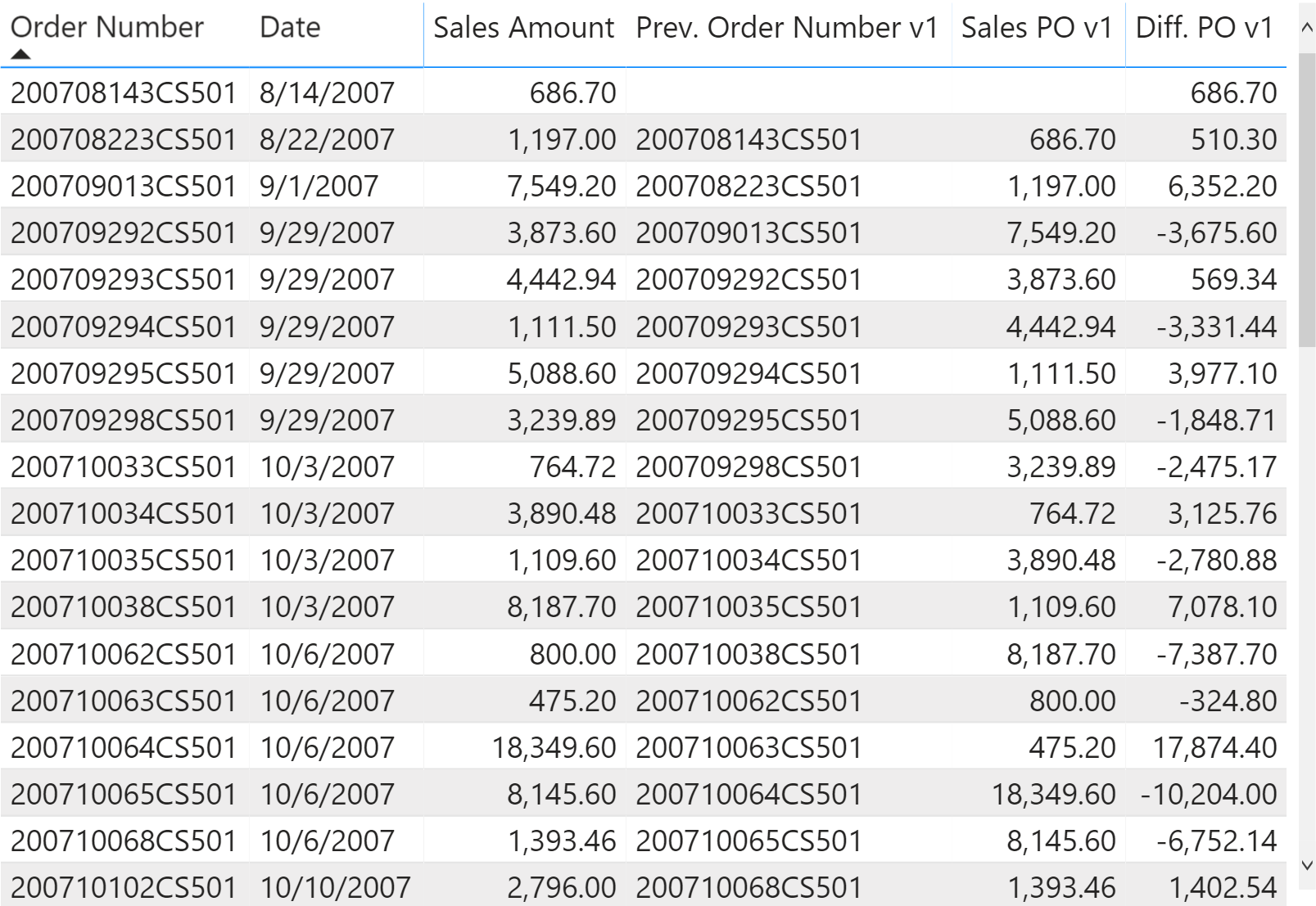
In this case the first task is to retrieve the previous order number. The following implementation uses LASTNONBLANK and removes the filter from Date in order to make sure to find the previous order also on other dates:
Prev. Order Number v1 :=
IF (
    NOT ISEMPTY ( Sales ),
    VAR FirstVisibleOrder =
        MIN ( Sales[Order Number] )
    VAR PreviousOrder =
        CALCULATE (
            LASTNONBLANK (
                DISTINCT ( Sales[Order Number] ),
                [Sales Amount]
            ),
            REMOVEFILTERS ( 'Date' ),
            Sales[Order Number] < FirstVisibleOrder
        )
    VAR Result =
        IF (
            NOT ISEMPTY ( Sales ),
            PreviousOrder
        )
    RETURN
        Result
)
From a performance standpoint, we prefer the implementation that uses a simple MAX aggregation:
Prev. Order Number v3 :=
IF (
    NOT ISEMPTY ( Sales ),
    VAR FirstVisibleOrder =
        MIN ( Sales[Order Number] )
    VAR PreviousOrder =
        CALCULATE (
            MAX ( Sales[Order Number] ),
            REMOVEFILTERS ( 'Date' ),
            Sales[Order Number] < FirstVisibleOrder
        )
    VAR Result =
        IF (
            NOT ISEMPTY ( Sales ),
            PreviousOrder
        )
    RETURN
        Result
)
In order to retrieve the Sales Amount of the previous order, the implementation based on LASTNONBLANKVALUE reduces the amount of code required:
Sales Previous Order v2 :=
VAR FirstVisibleOrder =
    MIN ( Sales[Order Number] )
VAR Result =
    CALCULATE (
        LASTNONBLANKVALUE (
            DISTINCT ( Sales[Order Number] ),
            [Sales Amount]
        ),
        REMOVEFILTERS ( 'Date' ),
        Sales[Order Number] < FirstVisibleOrder
    )
RETURN
    Result
This time the optimized version is more verbose, but this could provide a very important performance optimization!
Sales Previous Order v3 :=
VAR FirstVisibleOrder =
    MIN ( Sales[Order Number] )
VAR PreviousOrder =
    CALCULATE (
        MAX ( Sales[Order Number] ),
        REMOVEFILTERS ( 'Date' ),
        Sales[Order Number] < FirstVisibleOrder
    )
VAR FilterPreviousOrder =
    TREATAS (
        {
            PreviousOrder
        },
        Sales[Order Number]
    )
VAR Result =
    CALCULATE (
        [Sales Amount],
        REMOVEFILTERS ( 'Date' ),
        FilterPreviousOrder
    )
RETURN
    Result
Comparing query performance
The difference in performance between the different solutions depends on the cardinality applied by LASTNONBLANK (Date[Date] and Sales[Order Number] in our two scenarios) and the complexity of the measure being evaluated (Sales Amount). By filtering a single customer as we did in the examples shown in this article, it is hard to measure a difference because the execution time to refresh the report is below 10-20ms. For this reason, we created a benchmark query by removing the filter by customer so that we have more valid dates to compute. The measures considered are Sales PD and Sales PO, related to the corresponding scenarios. For each measure we used three versions:
- v1: using LASTNONBLANK
- v2: using LASTNONBLANKVALUE
- v3: using custom DAX
In order to benchmark the Sales PD scenario, we used the following query:
EVALUATE
TOPN (
    501,
    SUMMARIZECOLUMNS (
        'Date'[Date],
        "Sales_Amount", 'Sales'[Sales Amount],
        "Sales_PD", 'Sales'[Sales PD v1]    -- Change v1, v2, v3
    ),
    'Date'[Date], 1
)
ORDER BY 'Date'[Date]
The result obtained for Sales PD v1 using LASTNONBLANK is the following one. The cost of the storage engine is minimal and most of the operation are executed in the formula engine. A more complex measure or a bigger Sales table would affect the storage engine cost (the Sales table used in this example only contains 100,000 rows).

The same benchmark for Sales PD v2 using LASTNONBLANKVALUE displays an unexpectedly slower execution time. Thus, a simpler syntax does not necessarily translate to better performance.

Finally, the benchmark for Sales PD v3 (using custom DAX expressions) provides the best performance in terms of execution time.

The custom DAX formula reduces the execution time by 20% compared to v1 (LASTNONBLANK) and by 35% compared to v2 (LASTNONBLANKVALUE).
For the Sales PD scenario, we used the following query to perform the benchmark:
EVALUATE
TOPN (
    501,
    SUMMARIZECOLUMNS (
        'Sales'[Order Number],
        'Date'[Date],
        __DS0FilterTable,
        "Sales_Amount", 'Sales'[Sales Amount],
        "Sales_PO", 'Sales'[Sales PO v1]    -- Change v1, v2, v3
    ),
    'Sales'[Order Number], 1,
    'Date'[Date], 1
)
ORDER BY
    'Sales'[Order Number],
    'Date'[Date]
Because of the granularity of the Sales[Order Number] column, the execution is much slower in absolute terms compared to the previous scenario, showing a bigger difference between the different versions of the measures.
The result obtained for Sales PO v1 using LASTNONBLANK is the following one.

The result obtained for Sales PO v2 using LASTNONBLANKVALUE is the following one.

Finally, the Sales PO v3 measure provides the best execution time.

In this case the performance differences are only visible with a large granularity. The custom DAX formula reduces the execution time by 19% compared to v1 (LASTNONBLANK) and by 32% compared to v2 (LASTNONBLANKVALUE).
The differences shown might vary for different models and different queries. However, we do not expect to see cases where LASTNONBLANK or LASTNONBLANKVALUE are faster than the custom DAX solution. In some case, the differences are too small to be perceived by the report users.
Conclusion
The DAX functions FIRSTNONBLANK, FIRSTNONBLANKVALUE, LASTNONBLANK, and LASTNONBLANKVALUE are iterators that could materialize data at the granularity of the column provided as a first argument.
Most of the times, it is possible to get the same result by writing custom DAX code – code that might provide better performance and scalability thanks to a reduced level of materialization. In order to do so, it is necessary to make an assumption about the data model: the presence of transactions in the fact table (Sales in our example) is enough to consider the element iterated, without having to evaluate a measure to check whether it does or does not return a blank value.
While the difference in query performance may be small in simple reports, there could be a larger impact in complex reports.