This article describes how to analyze the performance of a DAX measure based on a DISTINCTCOUNT calculation and how to evaluate possible optimizations.
The VertiPaq engine is used by DAX when you query a model based on data loaded in memory. The performance of the Vertipaq engine is also outstanding when it counts unique values in a column using the DISTINCTCOUNT function. However, counting unique values in complex reports can still create performance issues. The main reason for this is that DISTINCTCOUNT is a non-additive aggregation that must be computed for every cell in the report. Understanding the behavior of this aggregation can explain why other equivalent expressions that are slower in theory, can provide better performance in specific reports.
This article shows how to implement the same DISTINCTCOUNT calculation in two alternative ways, measuring and comparing the performance in different reports. You will see that while DISTINCTCOUNT can be implemented using SUMX / DISTINCT, the DISTINCTCOUNT version is usually better. That is, unless the density of the reports is high and the calculation apply filters to the measures that do not correspond to the grouping granularity of the visualization – as is always the case using time intelligence functions. There are cases where SUMX / DISTINCT can offer better performance, but you have to clarify whether optimizing one report might slow down many others. Measuring performance using DAX Studio is the only way to know what to expect for your model and reports.
Measuring the performance of DISTINCTCOUNT
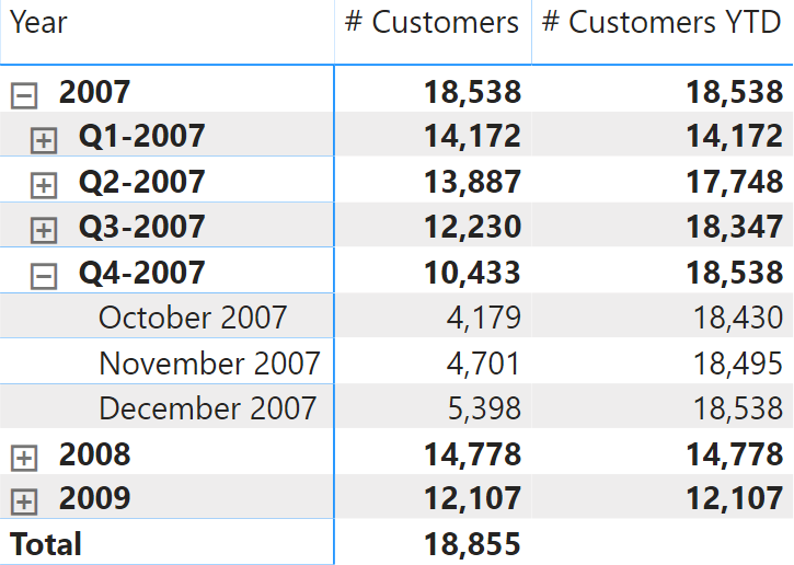
Consider a simple report using two measures to compute the number of unique customers buying a product: # Customers and # Customers YTD. The latter applies a year-to-date calculation to the former.
# Customers :=
DISTINCTCOUNT ( Sales[CustomerKey] )

# Customers YTD :=
CALCULATE (
    [# Customers],
    DATESYTD ( 'Date'[Date] )
)

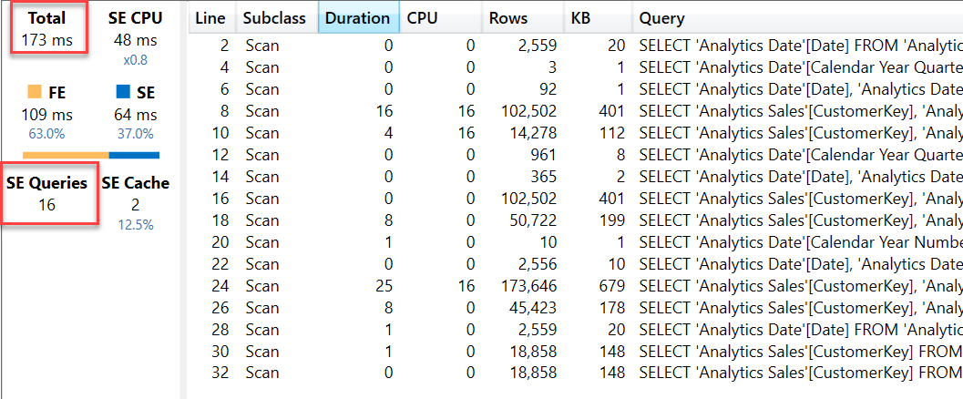
The execution of the DAX query generated for this visualization is relatively quick. However, it is interesting to see the large number of storage engine queries (SE Queries) executed in the query plan.

Because the distinct count calculation is non-additive, the result produced by the storage engine cannot be used by the formula engine to aggregate the result of an intermediate calculation. This is not an issue for a regular DISTINCTCOUNT measure, because there is a single SE query for each granularity level of the report. For example, this is the SE query visible at line 26 in the previous screenshot, corresponding to the calculation of the # Customers measure at the quarter granularity in 2007:
SELECT
    'Date'[Calendar Year Quarter Number],
    'Date'[Calendar Year Quarter],
    DCOUNT ( 'Sales'[CustomerKey] )
FROM 'Sales'
LEFT OUTER JOIN 'Date'
    ON 'Sales'[Order Date]='Date'[Date]
WHERE
    'Date'[Calendar Year Number] = 2007;
This single SE query returns 4 rows, corresponding to the result of # Customers for each of the quarters in 2017. However, sending a single SE query is not possible for the # Customers YTD calculation, which has a different filter context for each quarter produced by the DATESYTD function. Indeed, the three quarters are computed by the SE queries at line 14, 18, and 22 in the previous screenshot. The structure Each of each of these queries has a structure is similar to like the one used for the calculation of October 2007 (the xmSQL code has been simplified for readability purposes):
SELECT
    DCOUNT ( 'Sales'[CustomerKey] )
FROM 'Sales'
LEFT OUTER JOIN 'Date'
    ON 'Sales'[Order Date]='Date'[Date]
WHERE
    'Date'[Date] IN ( 39302.000000, 39094.000000, 39111.000000,..[304 total values, not all displayed] ) ;
Because every cell in the report has a different filter context made up of a different list of dates, it is not possible to create a single SE query that correctly describes the overlapping filters required for October 2007, November 2007, and December 2007.
Because this approach might seem expensive, we can consider the possible alternatives. DISTINCTCOUNT is just syntax sugar for a longer DAX expression using COUNTROWS and DISTINCT:
-- DISTINCTCOUNT internally uses COUNTROWS / DISTINCT
# Customers Basic :=
COUNTROWS ( DISTINCT ( Sales[CustomerKey] ) )
The query plan generated by the # Customers Basic measure is identical to # Customers and the two measures are semantically equivalent.
Measuring the performance of SUMX / DISTINCT
Another version of # Customers can be obtained by replacing COUNTROWS with SUMX, as in the # Customers SUMX measure:
# Customers SUMX :=
SUMX ( DISTINCT ( Sales[CustomerKey] ), 1 )

# Customers SUMX YTD :=
CALCULATE (
    [# Customers SUMX],
    DATESYTD ( 'Date'[Date] )
)
While the result of the # Customers SUMX measure is identical to that of # Customers, the request sent to the DAX engine is different: now there is an expression to compute for each unique value in Sales[CustomerKey]. The fact that this expression corresponds to the constant value of 1 is just a specific case. Now the query plan is different and more expensive, at least for the previous report.

This query runs in 173ms instead of the previous 101ms. The number of SE Queries was reduced, however this has not done much to reduce the overall amount of time spent in the storage engine (SE) which is still 64ms. The reason for the longer execution time is that the formula engine (FE) is consuming 63% of the total execution time. The SE queries at line 8, 16, and 24 have the following structure:
SELECT
    'Sales'[CustomerKey],
    'Date'[Date]
FROM 'Sales'
LEFT OUTER JOIN 'Date'
     ON 'Sales'[Order Date]='Date'[Date]
These SE queries materialize a list of customers and dates. The storage engine no longer aggregates data at the quarter level, this task is now in charge of the formula engine, which scans this list counting the number of unique values in the days that are included in the period (year, month, or quarter) displayed in each cell of the report.
Is this approach always slower? It depends.
If you had a report that displays a measure in many cells and if the number of unique values to compute were relatively small, then the situation could be different.
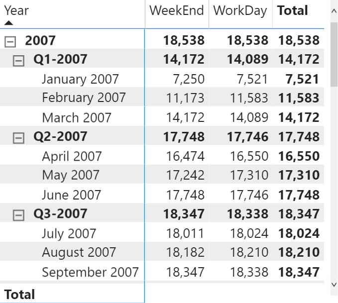
For example, consider a report where each cell has a different filter context that does not correspond to the grouping condition of the visualization. Most of the measures applying a time intelligence calculation present this condition. The following report uses the # Customers YTD measure in a matrix that groups the values by working day on the columns.

This time the version using the # Customers YTD measure is slower and produces a very large number of SE queries. Each SE query individually is fast, but the overhead for each query has a big impact on the overall result.

The report using # Customers YTD is 30% slower than the same report using # Customers SUMX YTD, but what is interesting is exploring the reasons why this happens. Pay attention to the smaller number of SE queries now being executed.

Usually we prefer a query plan that spends more time in the SE than in the FE. This is because the SE queries can be cached, whereas what is executed by the FE must be computed at every execution. However, when the number of SE queries produced by a single DAX query exceeds the limit of the SE queries kept in the cache (currently 256), then you no longer get any benefit from the VertiPaq cache.
Conclusions
We deliberately chose reports where the difference between these implementations was minimal, because we wanted to focus on the underlying behavior. There may be reports where the # Customer SUMX measure is way faster than the classic # Customer measure based on DISTINCTCOUNT, though usually the opposite is true.
These are the elements to consider when comparing DISTINCTCOUNT with the solution based on SUMX / DISTINCT:
- DISTINCTCOUNT relies more on the SE.
- The calculation of the result for a single cell in the result is usually faster using DISTINCTCOUNT.
- A measure with filters that differ for every cell regardless of the grouping conditions might require additional SE queries.
- A small number of SE queries may remain in the cache between calculations.
- The complexity of the report and the number of displayed cells with a DISTINCTCOUNT calculation might increase the number of SE queries.
- SUMX / DISTINCT materializes data to perform the calculation in the FE.
- A smaller number of SE queries is required.
- The materialization mightbe large, requiring more RAM at query time compared to DISTINCTCOUNT.
- The size of the materialization depends on the cardinality of the report and on the maximum number of unique values that could be computed based on the existing filters in the report.
You can see that the same model can produce different results in different reports. You should carefully consider the side effects of different implementations of DISTINCTCOUNT in order to avoid undesired side effects in other reports. The analysis of the query plans with DAX Studio can help predict the future behaviors of the same measure in different reports.